How to Clean Messy Data for Analysis in Excel Using Power Query?

How to clean messy data for analysis in Excel using Power Query? You have heard of Power Query and no doubt you have come across your fair share of messy data in Microsoft Excel. The question you might have asked yourself just how do you use Power Query to clean up messy data in Excel.

What this Excel Power Query tutorial covers:

• What makes messy data?
• What advantage is there to cleaning up messy data?
• How to get data into Power Query?

How to clean messy Excel Data for Analysis?

Are you needing to clean messy Excel Data? I know that you've been there. Your boss has given you a spreadsheet to analyse. It could look just like the following:

You have been asked to create charts using the above data. Wanting you to analyse by month, area and team.

If you try to select the data and create a chart, then this would be the result.

I think that you would agree that this chart is totally useless. The problem is one of summation. Bascially, you need to summarise the data before you create charts.

Before you can summarise this data, however, you'll need to re-structure the data in a format that Excel can work with. In other words you need to change the struction of the data into this:

Above is what you would called unpivoted data. In cleaning up messy data it is vital that you undertake this step. You see, the problem is that most people enter data into an Excel spreadsheet as they would expect to see it. They then try to bring the data into a Pivot Table or some other data analysis tool. Only to discover that it doesn't work.

What is Unpivoted Data?

In knowing how to clean messy data for analysis in Excel using Power Query, the Power Query part of that statement speaks of a part of Excel that sits unsung behind the scenes.

Power Query is the tool you will use to clean up, or unpivot, messy data. Unpivoting data is the process of changing data that cannot be analysed into a structure that can.

This tutorial will show how to do this, using common techniques that data analysts use to clean up this messy Excel data.

Importing Data into Excel

Now, let's import this messy Excel data into Power Query so that we can clean it up.

First thing to do is to delete that horrible chart, if you've followed along and insert it. Click on any white area near the border of the chart then press delete.

Selecting Data to Import to Power Query

The next thing on your list of tasks is to select the data that you want to import. This is how you do it:

1. Click anywhere in the data to import.
2. Hold Ctrl & End.
3. Hold Ctrl & Shift & Home.
4. Let go of the Ctrl key and with the Shift key held down tap the down arrow 3 times.

You should have selected the data that you'll import into Power Query.

Now that you have selected the data, it's time to import the data.

Importing the Data into Power Query

To import selected data into Power Query do the following:

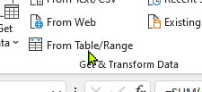
1. Click the Data tab at the top of the screen.
   
2. Click From Table/Range. (On the left).
   
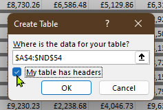
3. In the Create Table box select the My table has headers checkbox then Click OK.
   

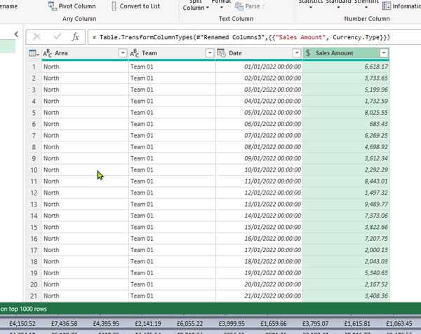
This will load the data into Power Query, looking like this:

Now it's time to use Power Query clean up the data so that we can analyse it.

Fill Down Blank Cells - Power Query

In knowing how to clean messy data for analysis in Excel using Power Query, it's necessary to know how to fill down data.

Look closely at the first column in the data.

You can see that the sales area has been imported. North, South, East and West. However, because the data in Excel had merged cells, Excel converted the data into a table. When that table was imported into Power Query those blank cells in the table were converted to nulls.

Fill down will convert all the nulls to the value at the top. This will ensure that data exists in all the rows for the area column. Do the following:

1. Ensure that Column1 is selected.
2. Click the Transform tab at the top.
   
3. Click the Fill Drop down menu, click Fill Down.
   
4. You can see that the Area column has now been filled down.
   
5. Double click on the column heading and type Area then press Enter.
   

Now that the area column has been filled you are well on your way to knowing how to clean messy data for analysis in Excel using Power Query. Next, we have to remove row and column totals.

Understanding the Applied Steps Feature in Power Query

If you look to the right of the screen you will see a section entitled "Applied Steps".

Understanding the Applied Steps section in Power Query is essential as there is no undo feature in Power Query.

So if you make a mistake you will use the Applied Steps section to remove that step by clicking on the cross to left to remove that step.

If you feel that you or your organisation could benefit from an Excel course then please check out either our instructor led live online Excel courses or face-to-face in person Excel training courses. Let our Excel trainers give you time saving hints and tips to help you and your colleagues optimise your Excel spreadsheets.

Removing Columns and Filtering Totals in Power Query

The next thing we'll do in cleaning up this messy Excel data is to remove the column and the row totals. We remove these totals because when we eventually load this data back into Excel, the Pivot Table or Chart that we will create from the data will do that automatically for us. By not removing the totals it would mean that the data would be inaccurate.

This is how to remove the totals (If you've been following from above):

1. Press End.
2. Right click on the Totals column and choose Remove.
   
3. The column has been removed.
4. Press Home to return back to the first column.
5. Click the filter drop-down list for Column2.
6. Remove the ticks from Totals.
   
7. Scroll up and remove the Tick from null.
   
8. Click OK.

Your data in Power Query should now look like this:

Double click on Column2 and change the name to Team, press enter.

Unpivoting Data in Power Query

Next, in knowing how to clean messy data for analysis in Excel using Power Query you'll have to get to grips with what's know as Unpivoting Data.

What is Unpivotted Data?

In the world of data analysis Unpivoted Data is data correctly structured. If you have a look at the data in Excel.

You can see that dates are across the top with the Areas and the Teams down the left hand side. This is what is called "Pivoted" data.

To be able to analyse the data we will have to unpivot the data, this is what you do:

How to Unpivot Data in Excel?

Right! Let's get to unpivotting this messy Excel data. Do the following:

1. Click on the Area column heading, hold down the shift key then click the Team column heading.
   
2. Next, click on the Unpivot Columns drop down menu at the top of the screen and choose Unpivot Other Columns.
   
3. Double click on the newly unpivoted data column, now called attribute, and rename it Date.
4. Use the data-type drop down menu to change the data type to Date/Time.
   
5. Rename the Value Column to Sales Amount, then change the data type to Currency.
   
6. Now your data is unpivoted and ready to be loaded back into Excel.

Loading Clean Data Back into Microsoft Excel

Now that you know how how to clean messy data for analysis in Excel using Power Query, the next stage to to load that newly cleaned data back into Excel.

Close and Load Data

You may have noticed that Power Query runs behind Excel. You can switch to Excel at any time. However, it's best practice to do what you need to do in Power Query then load the data back into Excel. This is how you do it:

1. Click on the Home Tab.
2. Click Close & Load then click Close & Load to..
   
3. Choose Table then click OK.
   
4. The data will be imported into Excel all clean and ready to go.

Analysing Excel Data with a Pivot Table and Pivot Chart

Now that you have cleaned your messy Excel data you can create a Pivot Table along with a Pivot Chart so that you can better be able to analyse the data.

Let's Create a Pivot Table

The first thing we'll do is to create a Pivot Table that will display the Sales Amount per Area.

Do the following:

1. Click once on the Table then click Table Design.
2. Now click on Summarise with Pivot Table.
3. Click OK.
   (A Pivot Table will be created on a new sheet in your Excel spreadsheet).
4. Using the PivotTable fields section on the right drag:
   1. Area to Rows
   2. Sales Amount to Values
5. The Pivot Table should look like this:
   

Changing the Number Format

There are a couple of changes that we need to make to the above PivotTable. One is that the list of area's are in the incorrect order. Before we handle this, however, we'll deal with the format of the numbers in the Sales Amount.

1. Right click on any number in the Sales Amount column.
2. Select Number Formatting.
3. Double Click on Accounting.
   
4. See that the formatting of the numbers on the Pivot Table have been updated.

Next thing that we need to do is to sort out the order of the areas. So that they read North, South, East and West in that order.

Be sure to check back to see how to do it.

The above is a typical example. Sometimes, however, you may find a little more is need to clean up your data. Make sure you check out our Power Query examples on Tiktok for more hints and tips on how to use Power Query.

Face to Face Power Query Consultancy

If you feel that you or your organisation could benefit from an Excel course then please check out either our instructor led live online Excel courses or face-to-face in person Excel training courses. Let our Excel trainers give you time saving hints and tips to help you and your colleagues optimise your Excel spreadsheets.

Other Excel Accounts Tutorials

Super Easy Accounts in Excel?

How to Make Your Spreadsheet Look Good?

Calculate VAT in Excel

Excel VAT Formula

Money Made Last Month

Pivot Tables for Beginners

Excel Financial Year Formula

Add Calculated Field to Pivot Table

Pivot Table Conditional Formatting

Excel Summary Sheet

SUMIF Excel Multiple Sheets

Clean up Messy Excel Data