Pivot Tables for Beginners Excel

Creating Pivot Tables for Beginners Excel

This Pivot Tables for beginners Excel tutorial will show you the basics of creating a Pivot Table. This tutorial is designed for those working with accounts. However, everyone can take advantage of this simple Pivot Tables guide.

If you've been creating an Excel accounts spreadsheet then you can do no worse than learn how to do a basic Pivot Table. Hence, this Pivot Tables for Beginners Excel tutorial will show you how to create a Pivot Table in the correct way.

First, you will see why using Tables is good practice in creating Pivot Tables. After that you will see how to add two Pivot Tables to a single sheet. Finally, you will learn how to connect a slicer which will allow you to control two Pivot Tables at the same time.

Should you want to follow along with this Pivot Tables tutorial then you can download the Pivot Tables for beginners exercise file.

If you can't wait and just want to access the Pivot Tables for beginners exercise file then download it here.

This tutorial is one of a series of Accounts Tutorials that you are encouraged to follow. As a result you will learn everything from creating a basic accounts worksheet to a Pivot Table. Also, you will learn many everyday Excel hints and tips.

Using Tables to Create Excel Pivot Tables

Create Tables - 0:56

Before you create a Pivot Table you should first know how and why you should create Tables in Excel. Using Tables to create Pivot Tables will benefit you by:

1. Make it easier to update your Pivot Table
2. Make your spreadsheet run faster
3. Make it easier to move your data and Pivot tables to different worksheets
4. Add easy to change colouring to your data

To create a table, click anywhere in the data from which you wish to create a table. Then click on Format as table from the Home tab on the Ribbon. Alternatively, you can use the Ctrl & T shortcut on the keyboard.

Then you can choose any colour theme you want. Then click OK.

Why give your Table a name?

By giving your Table a name in Excel you will find it easier to easily identify. Even though this is a Pivot Tables for beginners tutorial it is still a good practice. First you need to click anywhere in your data. After that you click on the Table Design tab on the Ribbon. The next step is to double-click the table name box, which you'll find in the top left of your screen. Finally, type in the name you want for your table and press Enter.

How do you Create the Pivot Table?

Create a Pivot Table - 2:29

Now you are ready to create your Pivot Table.

1. First thing is to click in any cell within your Table.
2. After that click on the Table Design tab at the top of the screen.
3. The next step is to click on the Summarize with Pivot Table button.
   
4. In the cell reference box you will see the name of the Table.
   
5. At the bottom click on the OK button.

Thus you have created your first Pivot Table. Moreover, even though you are a beginner, you have used the best method for beginners to create a Pivot Table.

Arranging a Pivot Table

Arranging Fields - 3:31

After creating your Pivot Table, you will need to arrange it to get it looking like you want it to. You do this by dragging the PivotTable fields to the Filters, Columns, Rows or Values boxes that you can see on the right of the screen.

First of all let's drag Received down to Values. As a result, the Pivot Tables displays the total amount received.

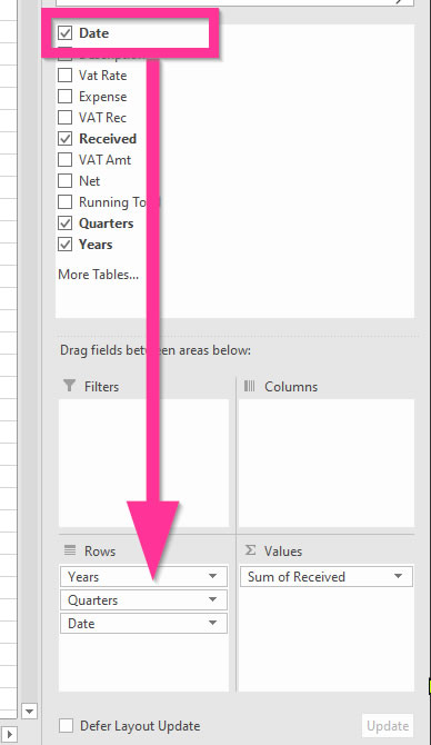
Now drag Date into Rows.

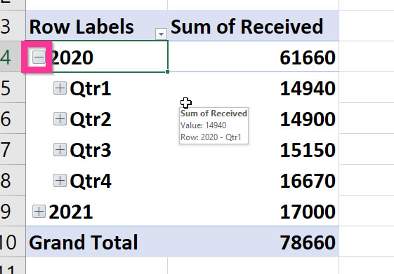
Note that the date has is displayed as a hierarchy. On later versions of Excel, date columns are automatically separated into date hierarchies of Years, Quarters, and Months depending on what time period your data covers.

As a result your Pivot Table has little expansion pluses you can click on to see more detail.

Excel Pivot Table Date Grouping

Date Grouping - 4:40

Presently, Excel has automatically arranged the dates in what is known as Excel Pivot Table Date Grouping. This means that dates that were originally entered as "01/01/2021" have now been grouping into respective Years, Quarters and Months. This is a Date Hierarchy and it can be changed.

To change the Pivot Table date grouping first, in the Pivot Table, right click on any date and select Group.

Now, in the Grouping box, choose the date grouping you want. For this example choose, Months and Years. You can do this by clicking on Quarters to deselect that grouping option. Then click OK.

As a result your Pivot will show dates grouped by months and years.

 

Change the Currency Format of Pivot Tables

Change Pivot Table Number Format - 6:50

Next, we will need to change the currency format of the Pivot Tables. As you can see the numbers under sum of received are unformatted therefore making them hard to read. As these numbers represent pounds and pence, we're going to change the format to currency.

Now, let's change the numbers. First, right click on any number in the Pivot Table then choose Number Format.

Second, in the Format Cells dialogue box select Accounting. Then click OK.

Why Accounting Format?

One of the reasons that I like to use the Accounting format to view monetary values in Excel is the fact that lines up the currency symbol to the left of the cell and that zero's are displayed as a dash.

How to Display a Summary of Expenses?

The next thing to do is to display a summary of Expenses using a Pivot Table. To do that, we are going to copy the Pivot Table that is already on the page, and paste it into cell D3.

Click any cell in the Pivot Table and then press Ctrl & A on the keyboard to select the Pivot Table.

Click in cell D3 and press Ctrl & V to paste a copy of the Pivot Table to the right of the first one.

Use the PivotTable Fields section to drag Expense to Values and Description to Rows.

Now, drag the Sum Of Received, Years and Date out of the field boxes to remove them from the Pivot Table.

Rows and Values should now look like the following picture.

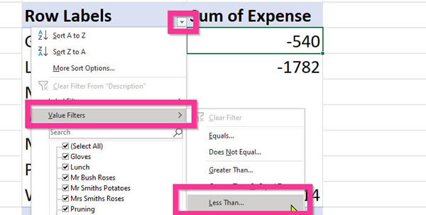
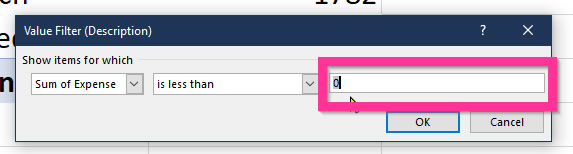
After you've done that, you will need to filter the Pivot Table to show only values below zero. Click on the Pivot Table filter menu and select Value Filters then Less Than.

In the Value Filter box type 0 to the right of the is less than box, then click OK.

The result is that the Pivot Table is now only showing negative values.

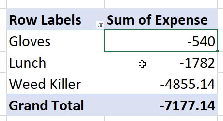
Next, we need to format the numbers as currency. So, right click any number then select Number Format. After that you need to click on Accounting and finally, click OK.

How to Connect Two Pivot Tables to One Slicer?

Connect Pivot Tables with Slicer - 7:52

Finally, we need to know how to connect two Pivot Tables to one slicer. In knowing this we will be able to filter both Pivot Tables at the same time.

To start of with, click on any month within the Pivot Table on the left.

Next, Click on the PivotTable Analyze tab on the Ribbon located at the top of the screen.

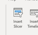
After that you need to click on the Insert Slicer button.

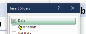
In the Insert Slicers box check Date then click OK.

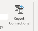
Next, click on Report Connections. You will find this on the Ribbon at the top of the screen.

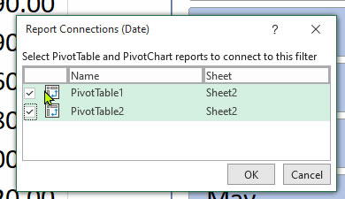
Finally, select the PivotTable2 checkbox, then click OK.

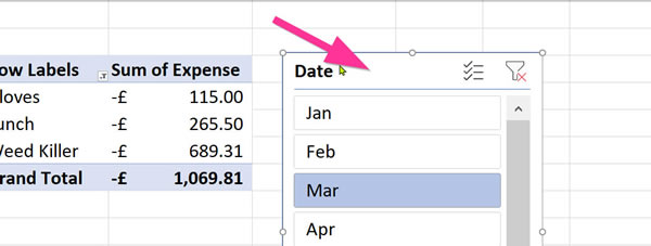
Next thing your should do is to drag your Slicer to the right of both the Pivot Tables. (You will need to use the Slicers header to drag as shown by the pink arrow in the below image).

You're finished! You've created a Pivot Table from your accounts spreadsheet. What’s more, you have also added Pivot Table Date Grouping along with viewing a summary of Expenses.

Moreover, you have also connected two Pivot Tables using a Slicer thereby allowing you to control two Pivot Tables at the same time.

This tutorial is part of a series of accounts tutorials which are designed for small businesses. It is hoped that by using them you can set up your accounts spreadsheets to make it easier for you to get the information you need.

Other Excel Accounts Tutorials