How Dynamic Highlighting Can Help You?
Are you tired of sifting through heaps of data, trying to find the information you need? Our step-by-step tutorial on how to dynamically highlight rows as you type in Excel is here to help! This practical guide will teach you how to search for data by typing, and as you do so, the relevant row containing that information will be highlighted automatically. Additionally, this tutorial includes the powerful wildcard search feature, which allows you to search for partial matches. This makes it even easier to locate the data you're after.
Data analysis can be overwhelming, particularly when working with large and intricate datasets. But worry not, as our comprehensive guide on how to dynamically highlight rows as you type in Excel is your solution. We'll walk you through the process of applying real-time formatting to your spreadsheets, enabling you to instantly locate the data you're searching for. Plus, you'll learn how to use wildcard searches, which help you find information even when you only remember a part of it. Say goodbye to tedious scrolling and embrace this transformative technique that will make your spreadsheets more efficient and interactive!
Dynamically highlighting rows
First thing you need to do is to download the dynamically highlighting rows exercise file so that you can follow along.
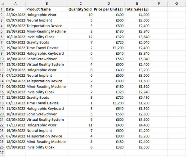
After you've opened the above exercise file adjust the column widths.
Now, insert 3 rows at the top. Highlight rows 1-3 then right-click and select insert.
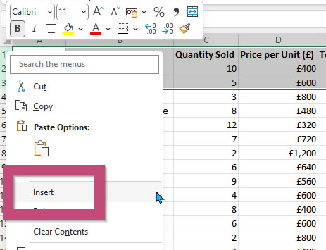
After that, you need to display the Developer tab. The Developer tab is the tab on the Ribbon you would use for forms and creating text boxes that can be edited.
To display the Developer tab right click any tab on the ribbon and choose customise the ribbon.
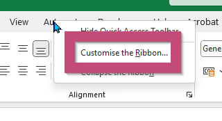
Check the developer tab.
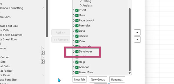
Once you have displayed the Developer tab, you need to draw a text box, click the Insert drop down list and click text box control.
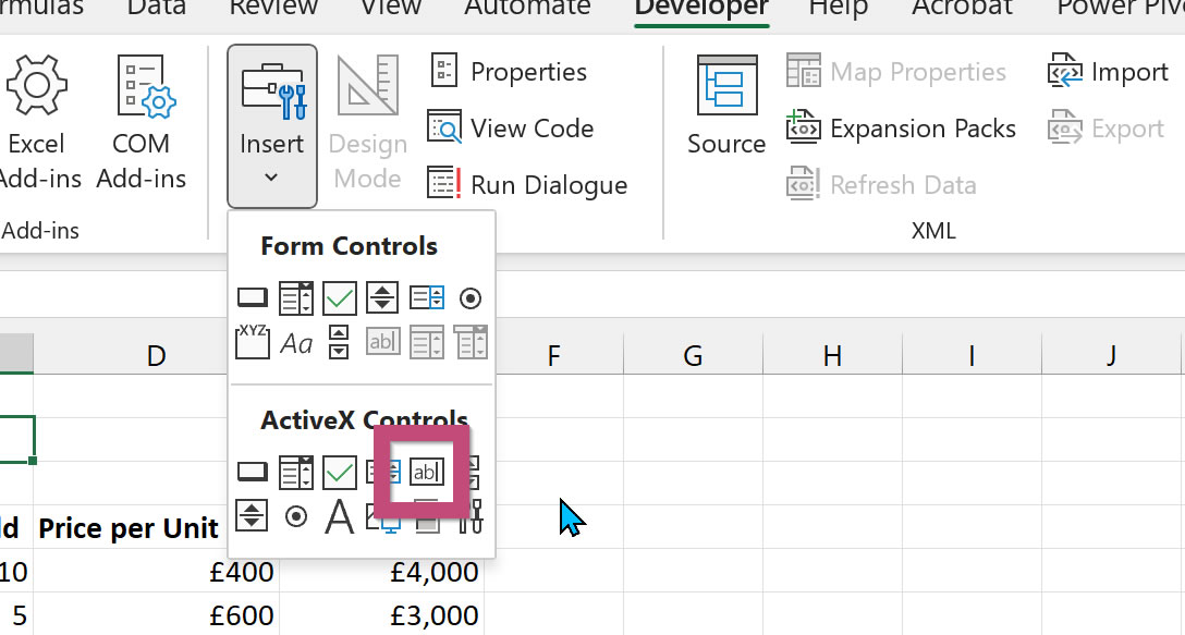
Right! Now draw a text box above the data.

Right-click on the newly drawn text box and choose properties.

In the Properties window for the text box, find the Linked Cell field and enter cell F1.

Great! Now, back on the Developer tab, click the Design Mode button to take Excel out of Design mode. Start typing in the Text box and see the text appear in cell F1. Amazing!

Dynamically highlight rows as you type
If you want to dynamically highlight rows as you type then next thing to do is to select the data you want highlighted. After that we'll go into conditional formatting. Let's do that.
Click anywhere in the data and press Ctrl & A to select all the data. Then click on Conditional Formatting and choose New Rule.
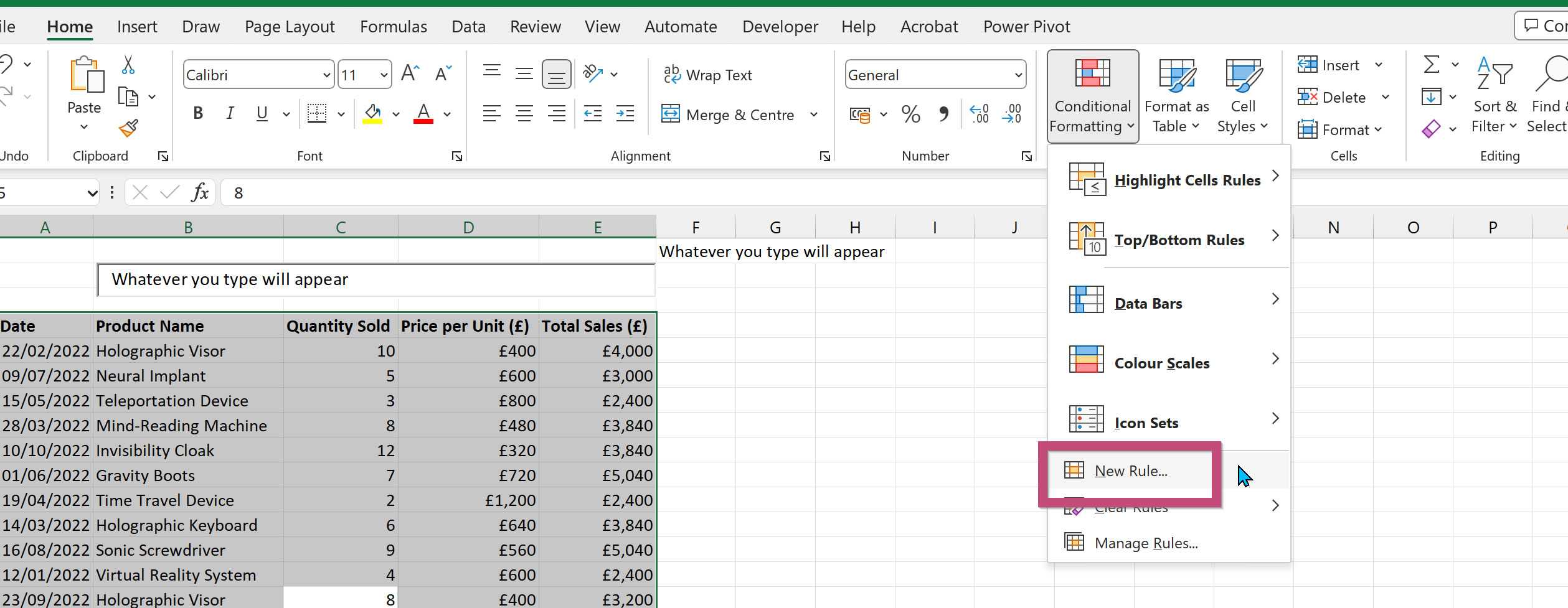
In the New Formatting Rules dialog box, select New formula and enter the following formula:
=AND(SEARCH($F$1,$B5),$F$1<>"")
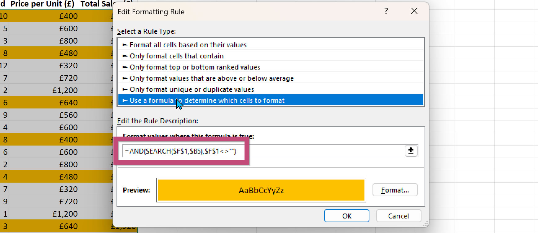
Then click format - fill colour - and choose the mustard yellow colour then click OK.
Now, type in the text box and see that the rows highlight.
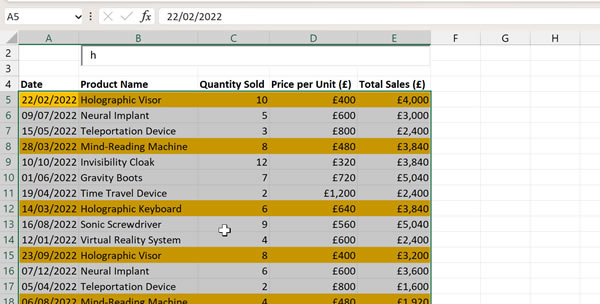
In this step-by-step guide, we provided detailed instructions on how to dynamically highlight rows as you type in Excel. We began by explaining the importance of this feature for managing and visualising large datasets. Next, we introduced conditional formatting rules and their role in achieving the desired outcome.
Throughout the guide, we followed a structured approach to ensure clarity and ease of understanding. We started by selecting the target data range, followed by creating a new conditional formatting rule using the formula-based option. We explained how to write the appropriate formula to highlight rows dynamically based on the input cell value. Finally, we demonstrated how to apply the rule and make necessary adjustments to ensure the desired results.
By following these instructions, users can now effortlessly implement dynamic row highlighting in their Excel spreadsheets, improving their overall data management experience.
There are extra details on the Microsoft website on conditional formatting that might be worth you checking out.
Other Excel Videos Tutorials


