Excel Financial Year Formula

Formula for Financial Year in Excel

The Excel financial year formula is a handy formula to work out the financial year in an Excel spreadsheet. Moreover, knowing how to calculate the financial year from a date allows you to analyse data by financial year.

Download: Starter file / Completed File

Financial Year Calculation

Financial Year Formula - 1:10

Use the following formula to calculate the financial year in Excel:

=IF(MONTH(A2)<4,YEAR(A2)-1 & "-" & YEAR(A2),YEAR(A2) & "-" & YEAR(A2)+1)

In the above example A2 contains the Date, the financial year formula is B2 and the date is 7th April 2021. The results should be:

For that extra little professional touch you add a right function to the second year in the formula to have only the last 2 digits of the year appear.

=IF(MONTH(A2)<4,YEAR(A2)-1 & "-" & RIGHT(YEAR(A2),2),YEAR(A2) & "-" & RIGHT(YEAR(A2)+1,2))

After you have entered in the formula you can Auto fill the formula down. Now you have something you can add to a Pivot Table and see how much money you made during the last financial year.

6th April Financial Year Formula

The above formula works if your company's financial year begins on the 1st of April. However, in the UK the financial year starts on the 6th of April.

This means we will need to add the DATE function to the formula like.

=IF(A2<=DATE(YEAR(A2),4,5),YEAR(A2)-1 & "-" & YEAR(A2),YEAR(A2) & "-" & YEAR(A2)+1)

The way this formula works is very similar to the other financial year formula however we are using the DATE function rather than MONTH to work out the financial year. Basically, if the date in cell A2 is less than April the 5th of the current year, we are in the previous financial year. Otherwise, we're in the next financial year.

Just one final touch to the formula, let's add the RIGHT function to finish it off.

=IF(A2<=DATE(YEAR(A2),4,5),YEAR(A2)-1 & "-" & RIGHT(YEAR(A2),2),YEAR(A2) & "-" & RIGHT(YEAR(A2)+1,2))

Here's how the formula looks in Excel. I place the formula on separate lines for readability. (Alt + Enter)

6th April UK Tax Year Formula for Financial Month

Once you've created the crazy calculation for financial year beginning 6th April, you'll need to work that into your financial month calculation. We can use a couple of methods. One is to split the year into 13 Periods of 28 days. As a word of explanation, this would equate to 13 periods of 28 days and the last period would be known as "Yearday" or Yearday2 in the case of a leap year. (Here is a blog about the 13 period year.).

You can use the following calculation for the 6th April tax year:

=TEXT(A2,"mmm") & " " & IF(A2<DATE(YEAR(A2),4,6),YEAR(A2)-1 & "/" & RIGHT(YEAR(A2),2),YEAR(A2) & "/" & RIGHT(YEAR(A2)+1,2))

How does the 6th April UK Tax Year Formula work?

The first part of the 6th April UK tax formula is:

=TEXT(A2,"mmm")

Extracts the abbreviated month name from the date. So, for example, if the date in cell A2 was 03/04/2021 the formula would return Apr.

The next part of the tax year formula looks like:

IF(A2<DATE(YEAR(A2),4,6),

This is the logical condition. This condition checks to see whether the date "A2" is currently less that the 6th of April. The YEAR(A2) part is checking the current year. If it is, then that date is counted as the previous financial year. If not (6th April onwards) the date is considered part of the next financial year. This can be see from the true part.

YEAR(A2)-1 & "/" & RIGHT(YEAR(A2),2),

So in the above formula, the date would return (2020/21) if the date was 3rd April 2021. This is because the 3rd of April is before the new tax year of the 6th April. Hence, it's included in the previous financial year calculation.

The false part of the IF function reads:

YEAR(A2) & "/" & RIGHT(YEAR(A2)+1,2)

Which would mean that the date 6th April 2021 would be shown as (2021/22) because the 6th April is after the cut off date for the new tax year. When you're finished you should have a sheet or a table that looks something like this:

So hopefully you're with me so far. You also, hopefully, can see that we've created something that we can use in a Pivot Table. So let's create a Pivot Table from Sales Amount.

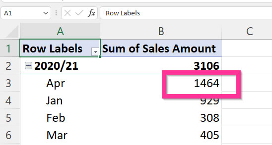
Nearly there! However, as you can see the sort order isn't correct. You've got Apr repeating 3 times at the top. That is because I have April figures across three years.

There's no definitive way to solve this issue. I've done a couple of methods. One is to create another Year column so that you can split the data on the Pivot Table like this:

Now the data you are seeing is from 6th April to 5th April. You can double check the figures by selecting them in the original data.

You can see, from the picture above, that I've selected the sales between the 1st and the 5th of April 2021. These sales consist of one sale on the 3rd April and 2 sales on the 5th April. If you look on the status bar below you can see that these sales add up to 1464.

Now, have a look at the Pivot Table, created earlier, you can see that the amount for that year is the same. It should be noted that there are no sales from 6th to the 30th April 2020. This issue will be addressed in the next section.

One final Pivot Table Grouping Issue

There is one final little snag. Notice that when displaying the month April within the year grouping levels there's no way of knowing whether the April is from the 6th to the 30th or 1st to 5th. So a little adjustment in the formula is required.

=TEXT(A2,"mmm") & IF(A2<DATE(YEAR(A2),4,6)," (1st - 5th April)","")

The bold bit that was added, checks to see if the date in the year is before the 6th April. In much the same way as we check the year, we use an if statement to check that the date is less than the 6th April of the current year` . If that's the case then we'll have the text (1st - 5th April) appear.

An age old problem

You can now see the difficulty of dealing with various dates. History has had numerous calendars used for dividing time. The above Excel financial tax year calculation is not a be all and end all answer to the issue. However, hopefully the above solution will give you an idea of how you can create your own Excel formula. I mean if you want to get technical and know how many days there are in a year the answer is:

365.242325 ephemeris days which equates to 365 days 5 hours 48 minutes 56.89s.

Hence I think we will be wrestling with this problem for a few centuries more.

Financial Quarter Calculation

Financial Quarter Calculation - 10:10

To find the financial quarter in a year you can use this formula:

="FQ-" & CHOOSE(MONTH(A2),4,4,4,1,1,1,2,2,2,3,3,3)

In the above formula the date is in cell A2. The formula first uses the MONTH function to get the month number from the date. After that the CHOOSE function will count along the list of numbers and give that number as a result. For instance if today's date is 7th April the MONTH is 4. Afterwards, the CHOOSE function will count, starting with the first number along to the fourth number, which is a 1, as seen below.

Finally, we concatenate or join the letters FQ to the start of the function. As a result you can see the financial Qtr.

Adding the Financial Year to a Pivot Table

Financial Quarter Calculation - 10:10

Now that you have created the financial year formula, you can add the colour to the Pivot Table.

If you haven't already done so covert your data range into a Table (Ctrl + T).

Click OK.

Next, Click on Summarize with PivotTable. You can find this button at the top of the screen.

Click OK.

Drag Financial Year into the Rows area and Received to the Values Area

You can now do the same with financial quarter.

Drag Date beneath Financial Qtr and remove Years and "Hey Presto!". You now have a Pivot Table display Financial Year, Quarters and the month is in the correct order.

Sorting Pivot Table by Financial Year

Using Custom Lists for Financial Year

How to Create a Custom List - 06:45

There is one more problem to overcome and that is if you remove the financial quarter, you will see that the order of the months revert back to January at the top and December at the bottom. We can use Custom Lists to overcome this problem.

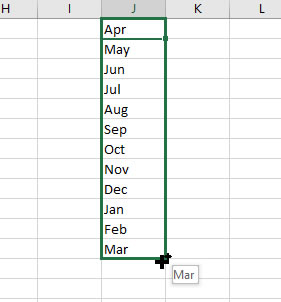
Click in any cell and type Apr.

Auto fill down to March.

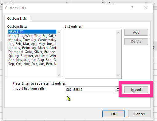
Next, go-to File - Options. Select Advanced from the left and then scroll all the way down to Custom Lists.

Click Import.

Click OK and OK again. (You can delete the original auto filled list from your spreadsheet).

Now, back in your Pivot Table, right click on any month and go to Sort then More Sort Options.

Click the More Options button then in the More Sort Options box untick Sort Automatically every time the report is updated and choose the Custom List you imported.

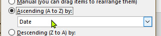
Click OK then in the Sort (Date) box choose Ascending by Date.

Click OK and you now have a financial year sorted by month without quarters. Plus, April is the first month.

In conclusion, the Excel financial year formula is just a piece of the puzzle. It's important you understand how to extract the financial quarter and change the sort order to give you accurate figures to analyse.

If you haven't already looked at the financial year tutorial then I really encourage you to do so.

Financial Year Using EOMonth

A nice simple formula to calculate the Financial year is to use the EOMONTH(A2,9). Then wrap that function in a year function so that the completed function looks like:

=YEAR(EOMONTH(A2,9))-1

Should you want to make it all clean and tidy. That is, having the financial year display as 2021/22 then you can use the following:

=YEAR(EOMONTH(A2,9))-1 & "-" & RIGHT(YEAR(EOMONTH(A2,9)),2)

This tutorial is one of a series of Accounts Tutorials that you are encouraged to follow. As a result you will learn everything from creating a basic accounts worksheet to a Pivot Table. Also, you will learn many everyday Excel hints and tips.

Other Excel Accounts Tutorials