Pivot Table Conditional Formatting

The Difference with Pivot Table Conditional Formatting is What?

At first Pivot Table Conditional Formatting may seem as straightforward as regular conditional formatting. For those who are wondering what conditional formatting is, it's when you change the colour of a cell based on a value. Also, conditional formatting can be used to display Icon's, change text colour or even show mini charts.

In this Pivot Table conditional formatting tutorial we will look at the proper way to use conditions in Excel to format data in a PivotTable. As a result you will be able to apply what you learn to your own Excel spreadsheets.

Pivot Table Conditional Formatting Training Content

• The Correct Way to do Pivot Table Conditional Formatting
• How to Apply Conditional Formatting to an Entire Row
• Allow Users to Change a Target Cell so that you Pivot Table Updates

Starter file - should you want to follow along. If, however, you want to jump to the end here is the completed file.

Best Way to do Pivot Table Conditional Formatting

Why Conditional Formatting in Pivot Tables isn't Working?

The main reason that Conditional Formatting with Pivot Tables doesn't work for most people is that they go about it the way they would usually go about Conditional Formatting in a spreadsheet. They, probably, would highlight the rows that they want to apply the Conditional Formatting to and click on the Conditional Formatting drop-down menu on the home tab. They might even think that it's working OK. That is until you filter the data or add a Slicer. Once you include a Slicer on your Pivot Tables or do any small amount of filtering, it will be painfully clear that Conditional Formatting is not working for you or your Pivot Tables.

The reason behind this is because instead of using cell references, which Conditional Formatting needs to work, Pivot Tables use the column headers of the source data to build the Pivot Table report. You may have notice that when you try to refer to a cell within a Pivot Table you get a weird GETPIVOTDATA function. So, obviously, when you try to use Conditional Formatting in a Pivot Table you encounter the same issue. (This tutorial will show how to add conditional formatting within a Pivot Table. If you want to use standard conditional formatting then check out this Microsoft Excel Support page on conditional formatting.

So What's the Proper Way to do Conditional Formatting in a Pivot Table?

So if you want to do Conditional Formatting in an Microsoft Excel Pivot Table the correct way, then you can apply the formatting to a single cell. After that, you can use the formatting options menu to apply the formatting to the entire field. However, there is one thing in which you need to be careful. Before you click on the Conditional Formatting menu in the Ribbon at the top of the screen, make sure that you select a cell in the Pivot Table that's within the grouping level you want to apply the Conditional Formatting to. If you want to know what I'm talking about, try the following. (Download the Exercise file first.)

1. Click Cell E6. (This contains the % Profit for the month of Jan. Because we selected this cell the Conditional Formatting will apply to the month grouping level. The month grouping level is indicated by the work date in the Rows section of the Pivot Table.)
2. From the Home Tab in the Styles section choose Conditional Formatting - Highlights Cells Rules - Less Than.
   
3. In the Less Than box type 90% then click OK.
   
4. Now use the Formatting Options menu in the right corner of Cell E6 to apply the Conditional Formatting to All Cells showing % Profit Values.
   

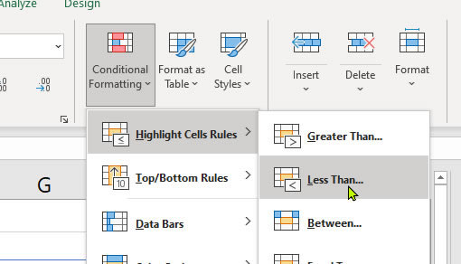
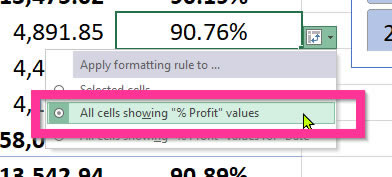
Now you can see that all values in the % Profit column that are below 90% are highlight in red. What is more you can filter the Pivot Table using the Slicer and it still works.

Pivot Table Conditional Formatting Entire Row

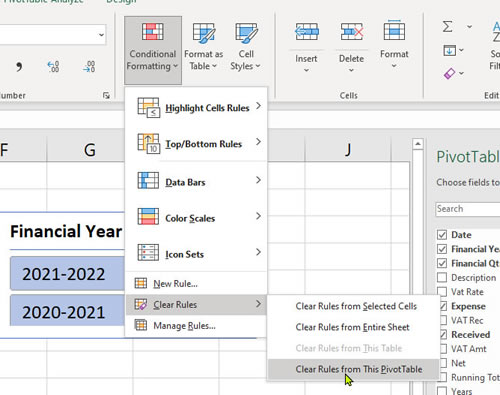
In Pivot Tables Conditional Formatting an entire row can be a little tricky. Because Pivot Tables are using the column headers in the source data, you can't use the dollar sign to copy the formula across. I'm afraid that you're going to have to do this manual. Or, at least, it's the only way I know how to do this. Before you carry out this exercise you'll have to delete the previous Conditional Formatting rule we set up in the last exercise.

How to Delete a Pivot Table Conditional Formatting Rule?

Here's how to delete a Pivot Table Conditional Formatting rule.

1. Click once on the Pivot Table that contains the rules you want to clear.
2. Conditional Formatting - Clear Rules - Clear Rules from this Pivot Table
   

How to Conditionally Format an Entire Row in a Pivot Table?

So now you're wondering how to conditionally format an entire row in a Pivot Table aren't you? First you need to create a Conditional Format based on a formula. Here's how to do it.

1. First select Cell E6.
2. Then click Conditional Formatting - New Rule.
3. After that select Use a formula to determine which cells to format.
4. Next select the All cells showing % Profit values for Date.
5. Then in the Format values where this formula is true box enter:
   =$E6<90%. (You can also use the mouse to click on the cell and use the F4 key to add the dollar symbol.)
6. After click Format.
7. Then select the Fill tab.
8. Now click on More Colours. Choose a red colour then click OK.
9. Next click OK again and your New Formatting Rule box should like the picture below.
   
10. After you're happy click OK.

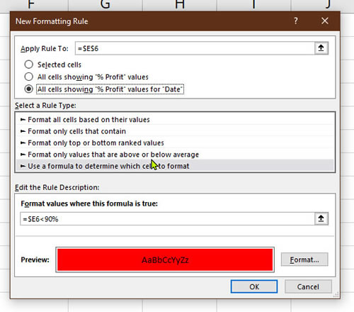
We're nearly finished. The last thing we need to do is to is copy, or duplicate, the Conditional Formatting rule to apply to the other columns in the Pivot Table.

1. Click Conditional Formatting - Manage Rules.
2. Click Duplicate Rule. (If the Duplicate Rule box doesn't appear it may be that you have an version of Excel older than 2019. If that is the case you will need to repeat the steps above this to create the same effect. In essence you will have to click on cell D6, applying conditional formatting as a formula. Then enter the formula as =$D6<90%. After that you will need to repeat for cell C6 and Cell B6.)
3. After you've duplicated the rule you can double click on the first rule in the list, which should be the one that has been duplicated, highlight whatever is in the Apply Rule to: box at the top and press delete on the keyboard. Then click on Cell D6 to select it.
   
4. Now click OK.
5. Repeat the above steps to apply to cells C6 and B6 then click Apply. You need to do this so that the Pivot Table can change the colour of the entire row. I'm sorry but I don't know how to change the colours of the months.
6. Finally click on OK and you should have a Pivot Table that is conditionally formatted along the entire row for any figures that are less than 90% in the % Profit column.
   

How to Apply Pivot Table Conditional Formatting Based on the Value of Another Cell?

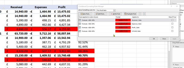
The last thing that we will do is to apply Conditional Formatting in our Pivot Table based up the value of another cell. As a result we will be able to set a target that can be updated with ease. Here is what you do:

1. In cell D1 enter the text Target and in E1 90%.
   
2. From the Ribbon select Conditional Formatting - Manage Rules.
3. Double click on the first rule in the list.
4. In the Format values where this formula is true box Replace the 90% with $E$1. (Simply highlight then click on the cell).
   
5. Click on OK.
6. Repeat the above for the other 3 Conditional Formatting rules.
   

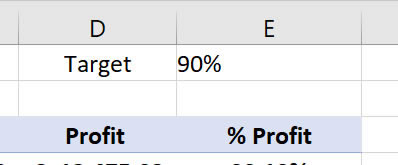
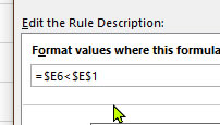
At last you're finished. In conclusion, it can be a real pain Conditionally Formatting in Pivot Tables. However, the effort is worth it. By knowing how to apply Pivot Table Conditional Formatting you can create KPI's within your Pivot Tables and bring your data to life.

• How to do Super Easy Accounts in Excel?
• How to make your Spreadsheets Look Good?
• Excel VAT Formula for different VAT rates

This tutorial is one of a series of Accounts Tutorials that you are encouraged to follow. As a result you will learn everything from creating a basic accounts worksheet to a Pivot Table. Also, you will learn many everyday Excel hints and tips.

Other Excel Accounts Tutorials

Super Easy Accounts in Excel?

How to Make Your Spreadsheet Look Good?

Calculate VAT in Excel

Excel VAT Formula

Money Made Last Month

Pivot Tables for Beginners

Excel Financial Year Formula

Add Calculated Field to Pivot Table

Pivot Table Conditional Formatting

Excel Summary Sheet

SUMIF Excel Multiple Sheets

Clean up Messy Excel Data