How to Make Spreadsheets Look Good

Making an Excel Spreadsheet Look Good

Make a Spreadsheet Look Good

If you want to know how to make spreadsheets look good the first thing you'll need to know is how to format an Excel spreadsheet. In fact to format a spreadsheet is the technical word used to describe how to make a spreadsheet look good.

Excel Spreadsheet - Download the Exercise File

The fundamentals of an accounting Excel spreadsheet is knowing basic spreadsheet formatting. This would include knowing how to change cells to currency in Excel, changing cell colour, and the rest of the standard formatting features within Microsoft Excel.

This tutorial is one of a series of Accounts Tutorials that you are encouraged to follow. As a result you will learn everything from creating a basic accounts worksheet to a Pivot Table. Also, you will learn many everyday Excel hints and tips.

Excel Accounts Template

If you are wanting to download then Excel Accounts Template that you will have created by the end of the tutorial, you are more that welcome to use the accounting template. However, please spend at least a few minutes watching the accounts tutorial, you'll get so much more out of it.

Also if watching an Excel accounts tutorial isn't for you and you would rather have step by step instructions then keep reading.

How to Insert a Row in Excel

Insert Row - 0:47

To start making your accounts look pretty in Excel the first thing to do would be to create a title. Knowing how to insert a row in Excel can help. Know it's true we covered that in the previous accounting tutorial in the series but just in case here's how to insert a row in an Excel spreadsheet.

1. Right Click on Row 1
2. Click Insert

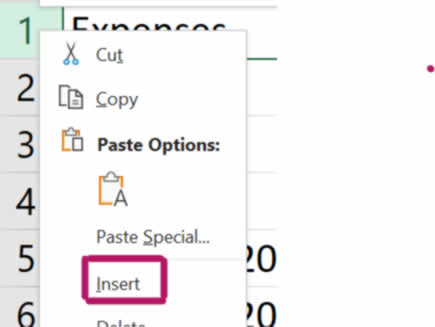
Notice that whenever you insert a row Excel always adds the row above the row you selected. To insert multiple rows in Excel simply drag down the number of rows you would like to insert. Then right click and click on Insert Row. Excel will insert as many rows as you selected.

Excel Insert Row Shortcut

Did you know that there's an Excel insert row shortcut? Try the following:

1. Click anywhere in Row 1 on the Spreadsheet
2. Shift & Space (Selects entire row)
3. Ctrl & Shift & + (Inserts row)

Merge and Centre Cells

Merge Cells - 1:00

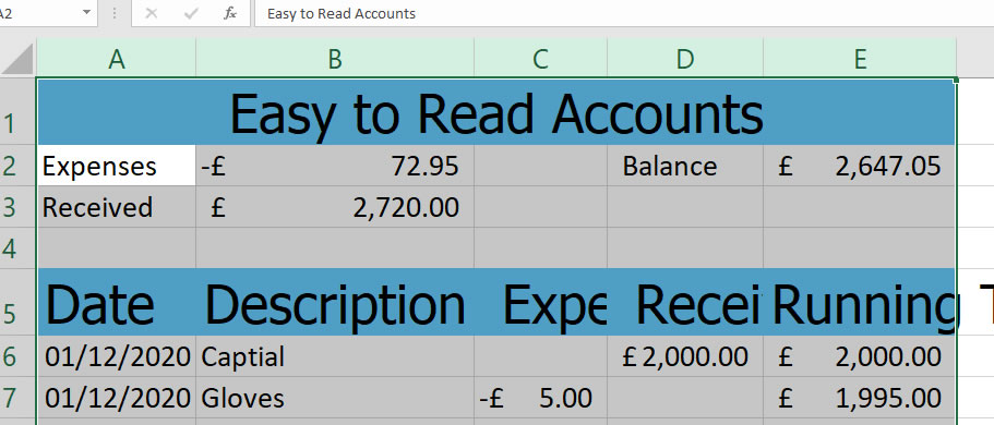
When you merge and centre cells you bring together a group of cells into one. Knowing how to merge multiple cells into one cell in Excel answers the question how do you add a title to an Excel spreadsheet? Here's how you do it:

1. Using the mouse select cells A1 - E1
2. Click on the Merge & Centre button on the ribbon at the top

3. Type the heading: "Easy to Read Accounts"

Now cells A1 through to E1 are merged into one cell. Notice that when you select the newly merged cell, it is given the cell reference A1. If you had data in any cell other that A1 you would lose the information. Excel will only keep any data you already had entered in cell A1.

Change Background Colour in Excel

Change Background Colour - 1:30

You can change the colour of cells in Excel. This not only makes the spreadsheet look pretty, it also makes your spreadsheet easy to read. Let's change the colour of our accounts spreadsheet:

1. Click Once on Cell A1
2. Click on the small triangle to the right of the paint bucket on the Ribbon at the top of the screen. (This is the cell fill colour button).

3. Click any colour you like

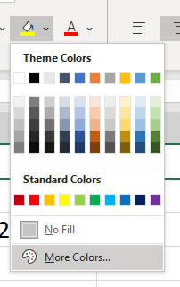
Now you can see that the background colour of cell A1 has changed. If you want to ensure the colours in your Excel spreadsheet match your company colours:

1. Select the Cells
2. Click Fill Colour Drop Down Arrow
3. Choose More Colours
4. Click Custom Tab at the Top
5. Enter the RGB or HEX values you've received from your companies marketing department

You can change the background colour of cells in Excel by selecting the cells before you change the background. Why not try to change the background colour of cells A5 to E5.

How to Change Font in Excel Sheet?

Change Font in Excel - 4:03

When you know how to change the font in the Excel Sheet you can really bring your accounts to life. In understanding how to do this you will first need to understand that the font will be changed for whatever cells are currently selected when you change the font in Excel. Here's how:

1. Click Cell A1. (This is the merged & centred title)
2. Click on the Font drop down list.

3. Select the font you like the look of by clicking on it.

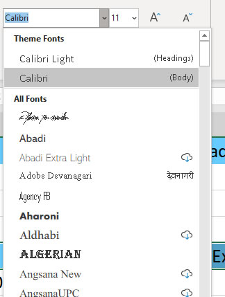
Note that as you move your mouse over the fonts the title updates to show you what the merged and centred title would look like in that particular font. Another tip is that you can search for a font you already know the name of by typing the font. I've chosen Tahoma for the Title and the column headings.

How to Change Font Size in Excel Spreadsheet

Change Font Size in Excel - 5:18

To change the font size in an Excel spreadsheet you would select the cells as described above. You would then use the Font Size drop down list to change the font size to the size you want.

You can also use the font size increase and decrease buttons if you just want to experiment. You don't have to accept the font sizes in the font size list. You can type any value you want into the font size box, even decimal numbers. So if you need your font to be 19.5 that's no problem. Simply type in the number you need.

How to Change the Width in Excel for Multiple Columns?

Adjust Width of Columns in Excel - 6:40

You probably already know how to change the width of one column in Excel. You might even know that you can change the width of a column automatically by double clicking on the line between the columns in the column headings. But did you know how to change column width in Excel for multiple columns? Well if you didn't here you go:

1. Select the Column Headings you want to Adjust

2. Double click on the dividing line between any of the column headers

How to Make Columns the Same Size in Excel?

If you want to know how to make columns the same size in Excel then you can do this:

1. Select Columns by their Headers
2. Double click any lines between the Column Headers

Hey presto! Your columns are the same width

Drawing Lines in Excel

Drawing Borders in Excel - 7:20

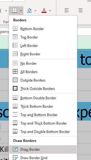
The quickest way to add borders to a worksheet is drawing lines in Excel. That's right you should know how to draw a border in Excel. Now how do you apply borders in Excel:

1. Click on the border drop down menu and choose Draw Border

2. Drag with the mouse to draw lines

How to Remove Lines in Excel?

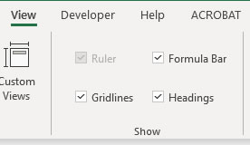
If you want to know how to remove lines in Excel then you at first need to know which lines. If you want to remove the grid lines you can do so by going to View on the Ribbon and unticking the Grid lines checkbox.

If, however, you wish to erase lines in Excel that you have drawn do the following:

1. Click the draw border drop down list
2. Click on the Erase button
3. Draw across the lines you want to erase

How to Fix the Top Rows in Excel

Fix Top Rows in Excel - 13:50

Knowing how to freeze panes in Excel means that you can fix rows or columns. Then you can scroll down the spreadsheet and still see the column headers. Try the following:

1. Click on the cell below the ones you want to freeze. So to rows 1 to 5 only as in the above tutorial you would click on cell A6.
2. From the Ribbon click the View Tab
3. Click Freeze Panes drop down list
4. Click Freeze Panes from the list

How to Create Alternative Row Colours in Excel?

Create Alternative Row Colours in Excel - 15:32

The Format painter button copies the format or look of currently selected cells. You can then select the cell or cells you wish to copy the formatting to. This is handy for one cell but absolutely fantastic for multiple cells. This is because you can use the format painter to create alternate coloured rows in Excel.

1. Select Cells A7 to E7.
2. Change the background colour to a light grey
3. Now Select Cells A6 to E7.
4. Click the Format Painter Button

5. Now select the rest of the cells down the sheet. Cells A8 to E119

Now your spreadsheet has alternate grey and white rows. See how handy knowing how you should use Format Painter is.

Simple Excel Accounts Template

Don't have time to follow the above tutorial? Here you go! This is the completed file: Simple Formatted Accounts Template.

Other Excel Accounts Tutorials

Super Easy Accounts in Excel?

How to Make Your Spreadsheet Look Good?

Calculate VAT in Excel

Excel VAT Formula

Money Made Last Month

Pivot Tables for Beginners

Excel Financial Year Formula

Add Calculated Field to Pivot Table

Pivot Table Conditional Formatting

Excel Summary Sheet

SUMIF Excel Multiple Sheets

Clean up Messy Excel Data